3. Program Flow
3.1. Hello, little turtles!
There are many modules in Python that provide very powerful features that we can use in our own programs. Some of these can send email, or fetch web pages. The one we’ll look at in this chapter allows us to create turtles and get them to draw shapes and patterns.
The turtles are fun, but the real purpose of the chapter is to teach ourselves a little more Python, and to develop our theme of computational thinking, or thinking like a computer scientist. Most of the Python covered here will be explored in more depth later.
3.1.1. Our first turtle program
Let’s write a couple of lines of Python program to create a new
turtle and start drawing a rectangle. (We’ll call the variable that
refers to our first turtle alex, but we can choose another
name if we follow the naming rules from the previous chapter).
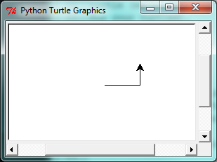
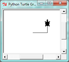
When we run this program, a new window pops up:
Here are a couple of things we’ll need to understand about this program.
The first line tells Python to load a module named turtle.
That module brings us two new types that we can use:
the Turtle type, and the Screen type. The dot
notation turtle.Turtle means “The Turtle type that is defined within
the turtle module”. (Remember that Python is case sensitive, so the
module name, with a lowercase t, is different from the type Turtle.)
We then create and open what it calls a screen (we would prefer to call it
a window), which we assign to variable window. Every window contains
a canvas, which is the area inside the window on which we can draw.
In line 3 we create a turtle. The variable alex is made to refer to this turtle.
So these first three lines have set things up, we’re ready to get our turtle to draw on our canvas.
In lines 5-7, we instruct the object alex to move, and to turn. We
do this by invoking, or activating, alex’s methods — these are
the instructions that all turtles know how to respond to.
The last line plays a part too: the window variable refers to
the window shown above. When we invoke its mainloop method, it enters
a state where it waits for events (like keypresses, or mouse movement and clicks).
The program will terminate when the user closes the window.
An object can have various methods — things it can do — and it can also have
attributes — (sometimes called properties). For example, each turtle has
a color attribute. The method invocation
alex.color("red") will make alex red, and drawing will be red too.
(Note the word color is spelled the American way!)
The color of the turtle, the width of its pen, the position of the turtle within the window, which way it is facing, and so on are all part of its current state. Similarly, the window object has a background color, and some text in the title bar, and a size and position on the screen. These are all part of the state of the window object.
Quite a number of methods exist that allow us to modify the turtle and the window objects. We’ll just show a couple. In this program we’ve only commented those lines that are different from the previous example (and we’ve used a different variable name for this turtle):
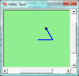
When we run this program, this new window pops up, and will remain on the screen until we close it.
Extend this program …
- Modify this program so that before it creates the window, it prompts the user to enter the desired background color. It should store the user’s responses in a variable, and modify the color of the window according to the user’s wishes. (Hint: you can find a list of permitted color names at http://www.tcl.tk/man/tcl8.4/TkCmd/colors.htm. It includes some quite unusual ones, like “peach puff” and “HotPink”.)
- Do similar changes to allow the user, at runtime, to set
tess’ color.
3.1.2. Instances — a herd of turtles
Just like we can have many different integers in a program, we can have many turtles.
Each of them is called an instance. Each instance has its own attributes and
methods — so alex might draw with a thin black pen and be at some position,
while tess might be going in her own direction with a fat pink pen.
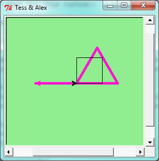
Here is what happens when alex completes his rectangle, and tess completes her triangle:
Here are some How to think like a computer scientist observations:
- There are 360 degrees in a full circle. If we add up all the turns that a turtle makes,
no matter what steps occurred between the turns, we can easily figure out if they
add up to some multiple of 360. This should convince us that
alexis facing in exactly the same direction as he was when he was first created. (Geometry conventions have 0 degrees facing East, and that is the case here too!) - We could have left out the last turn for
alex, but that would not have been as satisfying. If we’re asked to draw a closed shape like a square or a rectangle, it is a good idea to complete all the turns and to leave the turtle back where it started, facing the same direction as it started in. This makes reasoning about the program and composing chunks of code into bigger programs easier for us humans! - We did the same with
tess: she drew her triangle, and turned through a full 360 degrees. Then we turned her around and moved her aside. Even the blank line 18 is a hint about how the programmer’s mental chunking is working: in big terms,tess’ movements were chunked as “draw the triangle” (lines 12-17) and then “move away from the origin” (lines 19 and 20). - One of the key uses for comments is to record our mental chunking, and big ideas. They’re not always explicit in the code.
- And, uh-huh, two turtles may not be enough for a herd. But the important idea is that the turtle module gives us a kind of factory that lets us create as many turtles as we need. Each instance has its own state and behaviour.
3.1.3. The for loop
When we drew the square, it was quite tedious. We had to explicitly repeat the steps of moving and turning four times. If we were drawing a hexagon, or an octogon, or a polygon with 42 sides, it would have been worse.
So a basic building block of all programs is to be able to repeat some code, over and over again.
Python’s for loop solves this for us. Let’s say we have some friends, and we’d like to send them each an email inviting them to our party. We don’t quite know how to send email yet, so for the moment we’ll just print a message for each friend:
When we run this, the output looks like this:
Hi Joe.  Please come to my party!
Hi Zoe.  Please come to my party!
Hi Zuki.  Please come to my party!
Hi Thandi.  Please come to my party!
Hi Paris.  Please come to my party!
- The variable
friendin theforstatement at line 1 is called the loop variable. We could have chosen any other variable name instead, such asbroccoli: the computer doesn’t care. - Lines 2 and 3 are the loop body. The loop body is always indented. The indentation determines exactly what statements are “in the body of the loop”.
- On each iteration or pass of the loop, first a check is done to see if there are still more items to be processed. If there are none left (this is called the terminating condition of the loop), the loop has finished. Program execution continues at the next statement after the loop body, (e.g. in this case the next statement below the comment in line 4).
- If there are items still to be processed, the loop variable is updated to refer to the
next item in the list. This means, in this case, that the loop body is executed
here 7 times, and each time
friendwill refer to a different friend. - At the end of each execution of the body of the loop, Python returns
to the
forstatement, to see if there are more items to be handled, and to assign the next one tofriend.
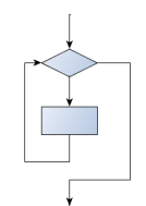
3.1.4. Flow of Execution of the for loop
As a program executes, the interpreter always keeps track of which statement is about to be executed. We call this the control flow, of the flow of execution of the program. When humans execute programs, they often use their finger to point to each statement in turn. So we could think of control flow as “Python’s moving finger”.
Control flow until now has been strictly
top to bottom, one statement at a time. The for loop changes this.
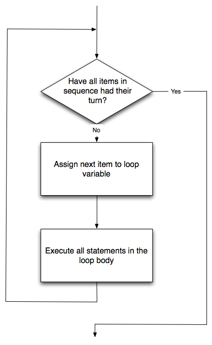
Flowchart of a for loop
Control flow is often easy to visualize and understand if we draw a flowchart.
This shows the exact steps and logic of how the for statement executes.
3.1.5. The loop simplifies our turtle program
To draw a square we’d like to do the same thing four times — move the turtle, and turn.
We previously used 8 lines to have alex draw the four sides of a square.
This does exactly the same, but using just three lines:
Some observations:
While “saving some lines of code” might be convenient, it is not the big deal here. What is much more important is that we’ve found a “repeating pattern” of statements, and reorganized our program to repeat the pattern. Finding the chunks and somehow getting our programs arranged around those chunks is a vital skill in computational thinking.
The values [0,1,2,3] were provided to make the loop body execute 4 times. We could have used any four values, but these are the conventional ones to use. In fact, they are so popular that Python gives us special built-in
rangeobjects:1 2 3 4
for i in range(4):
    # Executes the body with i = 0, then 1, then 2, then 3
for x in range(10):
    # Sets x to each of ... [0, 1, 2, 3, 4, 5, 6, 7, 8, 9]
Since we do not need or use the variable
iin this case, we could replace it with_, although this is not important for the program flow, it is good style.Computer scientists like to count from 0!
rangecan deliver a sequence of values to the loop variable in theforloop. They start at 0, and in these cases do not include the 4 or the 10.Our little trick earlier to make sure that
alexdid the final turn to complete 360 degrees has paid off: if we had not done that, then we would not have been able to use a loop for the fourth side of the square. It would have become a “special case”, different from the other sides. When possible, we’d much prefer to make our code fit a general pattern, rather than have to create a special case.
So to repeat something four times, a good Python programmer would do this:
By now you should be able to see how to change our previous program so that
tess can also use a for loop to draw her equilateral triangle.
But now, what would happen if we made this change?
A variable can also be assigned a value that is a list. So lists can also be used in
more general situations, not only in the for loop. The code above could be rewritten like this:
- Notice the difference between the method
alex.color, which is “part of” the instancealex, and the variablecolor, which is “part of” the main body of your program.
3.1.6. A few more turtle methods and tricks
Turtle methods can use negative angles or distances. So tess.forward(-100)
will move tess backwards, and tess.left(-30) turns her to the right. Additionally,
because there are 360 degrees in a circle, turning 30 to the left will get tess facing
in the same direction as turning 330 to the right! (The on-screen animation will differ,
though — you will be able to tell if tess is turning clockwise or counter-clockwise!)
This suggests that we don’t need both a left and a right turn method — we could be
minimalists, and just have one method. There is also a backward
method. (If you are very nerdy, you might enjoy saying alex.backward(-100) to
move alex forward!)
Part of thinking like a scientist is to understand more of the structure and rich relationships in our field. So revising a few basic facts about geometry and number lines, and spotting the relationships between left, right, backward, forward, negative and positive distances or angles values is a good start if we’re going to play with turtles.
A turtle’s pen can be picked up or put down. This allows us to move a turtle to a different place without drawing a line. The methods are
Every turtle can have its own shape. The ones available “out of the box”
are arrow, blank, circle, classic, square, triangle, turtle.
We can speed up or slow down the turtle’s animation speed. (Animation controls how quickly the turtle turns and moves forward). Speed settings can be set between 1 (slowest) to 10 (fastest). But if we set the speed to 0, it has a special meaning — turn off animation and go as fast as possible.
A turtle can “stamp” its footprint onto the canvas, and this will remain after the turtle has moved somewhere else. Stamping works, even when the pen is up.
Let’s do an example that shows off some of these new features:
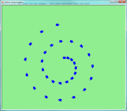
Be careful now! How many times was the body of the loop executed? How many turtle
images do we see on the screen? All except one of the shapes we see on the screen here
are footprints created by stamp. But the program still only has one turtle
instance — can you figure out which one here is the real tess? (Hint: if you’re not
sure, write a new line of code after the for loop to change tess’ color,
or to put her pen down and draw a line, or to change her shape, etc.)
3.2. Conditionals
Programs get really interesting when we can test conditions and change the program behaviour depending on the outcome of the tests. That’s what this part is about.
3.2.1. Boolean values and expressions
A Boolean value is either true or false. It is named after the British mathematician, George Boole, who first formulated Boolean algebra — some rules for reasoning about and combining these values. This is the basis of all modern computer logic.
In Python, the two Boolean values are True and False (the
capitalization must be exactly as shown), and the Python type is bool.
>>> type(True)
<class 'bool'>
>>> type(true)
Traceback (most recent call last):
  File "<interactive input>", line 1, in <module>
NameError: name 'true' is not defined
A Boolean expression is an expression that evaluates to produce a result which is
a Boolean value. For example, the operator == tests if two values are equal.
It produces (or yields) a Boolean value:
>>> 5 == (3 + 2)   # Is five equal 5 to the result of 3 + 2?
True
>>> 5 == 6
False
>>> j = "hel"
>>> j + "lo" == "hello"
True
In the first statement, the two operands evaluate to equal values, so the expression evaluates
to True; in the second statement, 5 is not equal to 6, so we get False.
The == operator is one of six common comparison operators which all produce
a bool result; here are all six:
x == y               # Produce True if ... x is equal to y
x != y               # ... x is not equal to y
x > y                # ... x is greater than y
x < y                # ... x is less than y
x >= y               # ... x is greater than or equal to y
x <= y               # ... x is less than or equal to y
Although these operations are probably familiar, the Python symbols are
different from the mathematical symbols. A common error is to use a single
equal sign (=) instead of a double equal sign (==). Remember that =
is an assignment operator and == is a comparison operator. Also, there is
no such thing as =< or =>.
Like any other types we’ve seen so far, Boolean values can be assigned to variables, printed, etc.
>>> age = 19
>>> old_enough_to_get_driving_licence = age >= 18
>>> print(old_enough_to_get_driving_licence)
True
>>> type(old_enough_to_get_driving_licence)
<class 'bool'>
3.2.2. Logical operators
There are three logical operators, and, or, and not,
that allow us to build more complex
Boolean expressions from simpler Boolean expressions. The
semantics (meaning) of these operators is similar to their meaning in English.
For example, x > 0 and x < 10 produces True only if x is greater than 0 and
at the same time, x is less than 10.
n % 2 == 0 or n % 3 == 0 is True if either of the conditions is True,
that is, if the number n is divisible by 2 or it is divisible by 3. (What do
you think happens if n is divisible by both 2 and by 3 at the same time?
Will the expression yield True or False? Try it in your Python interpreter.)
Finally, the not operator negates a Boolean value, so not (x > y)
is True if (x > y) is False, that is, if x is less than or equal to
y. In other words: not True is False, and not False is True.
The expression on the left of the or operator is evaluated first: if the result is True,
Python does not (and need not) evaluate the expression on the right — this is called short-circuit evaluation.
Similarly, for the and operator, if the expression on the left yields False, Python does not
evaluate the expression on the right.
So there are no unnecessary evaluations.
3.2.3. Truth Tables
A truth table is a small table that allows us to list all the possible inputs,
and to give the results for the logical operators. Because the and and or
operators each have two operands, there are only four rows in a truth table that
describes the semantics of and.
a b a and b False False False False True False True False False True True True
In a Truth Table, we sometimes use T and F as shorthand for the two
Boolean values: here is the truth table describing or:
a b a or b F F F F T T T F T T T T
The third logical operator, not, only takes a single operand, so its truth table
only has two rows:
a not a F T T F
3.2.4. Simplifying Boolean Expressions
A set of rules for simplifying and rearranging expressions is called an algebra. For example, we are all familiar with school algebra rules, such as:
n * 0 == 0
Here we see a different algebra — the Boolean algebra — which provides rules for working with Boolean values.
First, the and operator:
x and False == False
False and x == False
y and x == x and y
x and True == x
True and x == x
x and x == x
Here are some corresponding rules for the or operator:
x or False == x
False or x == x
y or x == x or y
x or True == True
True or x == True
x or x == x
Two not operators cancel each other:
not (not x) == x
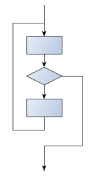
3.2.5. Conditional execution
In order to write useful programs, we almost always need the ability to check conditions and change the behavior of the program accordingly. Conditional statements give us this ability. The simplest form is the if statement:
The Boolean expression after the if statement is called the condition.
If it is true, then all the indented statements get executed. If not, then all
the statements indented under the else clause get executed.
Flowchart of an if statement with an else clause
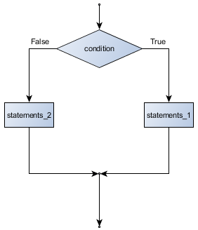
The syntax for an if statement looks like this:
As with the function definition from the next chapter and other compound
statements like for, the if statement consists of a header line and a body. The header
line begins with the keyword if followed by a Boolean expression and ends with
a colon (:).
The indented statements that follow are called a block. The first unindented statement marks the end of the block.
Each of the statements inside the first block of statements are executed in order if the Boolean
expression evaluates to True. The entire first block of statements
is skipped if the Boolean expression evaluates to False, and instead
all the statements indented under the else clause are executed.
There is no limit on the number of statements that can appear under the two clauses of an
if statement, but there has to be at least one statement in each block. Occasionally, it is useful
to have a section with no statements (usually as a place keeper, or scaffolding,
for code we haven’t written yet). In that case, we can use the pass statement, which
does nothing except act as a placeholder.
3.2.6. Omitting the else clause
Flowchart of an if statement with no else clause
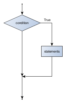
Another form of the if statement is one in which the else clause is omitted entirely.
In this case, when the condition evaluates to True, the statements are
executed, otherwise the flow of execution continues to the statement after the if.
In this case, the print function that outputs the square root is the one after the if — not
because we left a blank line, but because of the way the code is indented. Note too that
the function call math.sqrt(x) will give an error unless we have an import math statement,
usually placed near the top of our script.
Python terminology
Python documentation sometimes uses the term suite of statements to mean what we have called a block here. They mean the same thing, and since most other languages and computer scientists use the word block, we’ll stick with that.
Notice too that else is not a statement. The if statement has
two clauses, one of which is the (optional) else clause.
3.2.7. Chained conditionals
Sometimes there are more than two possibilities and we need more than two branches. One way to express a computation like that is a chained conditional:
Flowchart of this chained conditional
elif is an abbreviation of else if. Again, exactly one branch will be
executed. There is no limit of the number of elif statements but only a
single (and optional) final else statement is allowed and it must be the last
branch in the statement:
Each condition is checked in order. If the first is false, the next is checked, and so on. If one of them is true, the corresponding branch executes, and the statement ends. Even if more than one condition is true, only the first true branch executes.
3.2.8. Nested conditionals
One conditional can also be nested within another. (It is the same theme of composability, again!) We could have written the previous example as follows:
Flowchart of this nested conditional
The outer conditional contains two branches.
The second branch contains another if statement, which
has two branches of its own. Those two branches could contain
conditional statements as well.
Although the indentation of the statements makes the structure apparent, nested conditionals very quickly become very difficult to read. In general, it is a good idea to avoid them when we can.
Logical operators often provide a way to simplify nested conditional statements. For example, we can rewrite the following code using a single conditional:
The print function is called only if we make it past both the
conditionals, so instead of the above which uses two if statements each with
a simple condition, we could make a more complex condition using the and operator. Now we only
need a single if statement:
In this case there is a third option:
3.2.9. Logical opposites
Each of the six relational operators has a logical opposite: for example, suppose we can get a driving licence when our age is greater or equal to 18, we can not get the driving licence when we are less than 18.
Notice that the opposite of >= is <.
operator logical opposite == != != == < >= <= > > <= >= <
Understanding these logical opposites allows us to sometimes get rid of not
operators. not operators are often quite difficult to read in computer code, and
our intentions will usually be clearer if we can eliminate them.
For example, if we wrote this Python:
it would probably be clearer to use the simplification laws, and to write instead:
Two powerful simplification laws (called de Morgan’s laws) that are often helpful when dealing with complicated Boolean expressions are:
(not (x and y))  ==  ((not x) or (not y))
(not (x or y))   ==  ((not x) and (not y))
For example, suppose we can slay the dragon only if our magic lightsabre sword is charged to 90% or higher, and we have 100 or more energy units in our protective shield. We find this fragment of Python code in the game:
de Morgan’s laws together with the logical opposites would let us rework the condition in a (perhaps) easier to understand way like this:
We could also get rid of the not by swapping around the then and
else parts of the conditional. So here is a third version, also equivalent:
To improve readability, there is this fourth version:
This version is probably the best of the four, because it very closely matches the initial English statement. Clarity of our code (for other humans), and making it easy to see that the code does what was expected should always be highest priority.
As our programming skills develop we’ll find we have more than one way to solve any problem. So good programs are designed. We make choices that favour clarity, simplicity, and elegance. The job title software architect says a lot about what we do — we are architects who engineer our products to balance beauty, functionality, simplicity and clarity in our creations.
Tip
Once our program works, we should play around a bit trying to polish it up. Write good comments. Think about whether the code would be clearer with different variable names. Could we have done it more elegantly? Should we rather use a function? Can we simplify the conditionals?
We think of our code as our creation, our work of art! We make it great.
3.3. Iteration
Computers are often used to automate repetitive tasks. Repeating identical or similar tasks without making errors is something that computers do well and people do poorly.
Repeated execution of a set of statements is called iteration. Because
iteration is so common, Python provides several language features to make it
easier. We’ve already seen the for statement. This is the form of
iteration you’ll likely be using most often. But here we’re going to look
at the while statement — another way to have your program do iteration,
useful in slightly different circumstances.
Before we do that, let’s just review a few ideas…
3.3.1. Assignment
As we have mentioned previously, it is legal to make more than one assignment to the same variable. A new assignment makes an existing variable refer to a new value (and stop referring to the old value).
The output of this program is:
15
7
because the first time airtime_remaining is
printed, its value is 15, and the second time, its value is 7.
It is especially important to distinguish between an
assignment statement and a Boolean expression that tests for equality.
Because Python uses the equal token (=) for assignment,
it is tempting to interpret a statement like
a = b as a Boolean test. Unlike mathematics, it is not! Remember that the Python token
for the equality operator is ==.
Note too that an equality test is symmetric, but assignment is not. For example,
if a == 7 then 7 == a. But in Python, the statement a = 7
is legal and 7 = a is not.
In Python, an assignment statement can make two variables equal, but because further assignments can change either of them, they don’t have to stay that way:
The third line changes the value of a but does not change the value of
b, so they are no longer equal. (In some programming languages, a different
symbol is used for assignment, such as <- or :=, to avoid confusion. Some
people also think that variable was an unfortunae word to choose, and instead
we should have called them assignables. Python chooses to
follow common terminology and token usage, also found in languages like C, C++, Java, and C#,
so we use the tokens = for assignment, == for equality, and we talk of variables.
3.3.2. Updating variables
When an assignment statement is executed, the right-hand side expression (i.e. the expression that comes after the assignment token) is evaluated first. This produces a value. Then the assignment is made, so that the variable on the left-hand side now refers to the new value.
One of the most common forms of assignment is an update, where the new value of the variable depends on its old value. Deduct 40 cents from my airtime balance, or add one run to the scoreboard.
Line 2 means get the current value of n, multiply it by three and add
one, and assign the answer to n, thus making n refer to the value.
So after executing the two lines above, n will point/refer to the
integer 16.
If you try to get the value of a variable that has never been assigned to, you’ll get an error:
>>> w = x + 1
Traceback (most recent call last):
  File "<interactive input>", line 1, in
NameError: name 'x' is not defined
Before you can update a variable, you have to initialize it to some starting value, usually with a simple assignment:
Line 3 — updating a variable by adding 1 to it — is very common.
It is called an increment of the variable; subtracting 1 is called a decrement.
Sometimes programmers also talk about bumping a variable, which means the same
as incrementing it by 1. This is commonly done with the += operator.
3.3.3. The for loop revisited
Recall that the for loop processes each item in a list. Each item in
turn is (re-)assigned to the loop variable, and the body of the loop is executed.
We saw this example before:
Running through all the items in a list is called traversing the list, or traversal.
Let us write some code now to sum up all the elements in a list of numbers. Do this by hand first, and try to isolate exactly what steps you take. You’ll find you need to keep some “running total” of the sum so far, either on a piece of paper, in your head, or in your calculator. Remembering things from one step to the next is precisely why we have variables in a program: so we’ll need some variable to remember the “running total”. It should be initialized with a value of zero, and then we need to traverse the items in the list. For each item, we’ll want to update the running total by adding the next number to it.
3.3.4. The while statement
Here is a fragment of code that demonstrates the use of the while statement:
You can almost read the while statement as if it were English. It means,
while i is less than or equal to n, continue executing the body of the loop. Within
the body, each time, increment i. When i passes n, return your accumulated sum.
In other words: while <CONDITION> is True, <STATEMENT> is executed.
Of course, this example could be written more concisely as sum(range(n + 1)) because the function sum already exists.
More formally, here is precise flow of execution for a while statement:
- Evaluate the condition at line 5, yielding a value which is either
FalseorTrue. - If the value is
False, exit thewhilestatement and continue execution at the next statement (line 8 in this case). - If the value is
True, execute each of the statements in the body (lines 6 and 7) and then go back to thewhilestatement at line 5.
The body consists of all of the statements indented below the while keyword.
Notice that if the loop condition is False the first time we get
loop, the statements in the body of the loop are never executed.
The body of the loop should change the value of one or more variables so that eventually the condition becomes false and the loop terminates. Otherwise the loop will repeat forever, which is called an infinite loop.
In the case here, we can prove that the loop terminates because we
know that the value of n is finite, and we can see that the value of i
increments each time through the loop, so eventually it will have to exceed n. In
other cases it is not so easy, maybe even impossible, to tell if the loop will ever
terminate.
What you will notice here is that the while loop is more work for
you — the programmer — than the equivalent for loop. When using a while
loop one has to manage the loop variable yourself: give it an initial value, test
for completion, and then make sure you change something in the body so that the loop
terminates. By comparison, here is an equivalent snippet that uses for instead:
Notice the slightly tricky call to the range function — we had to add one onto n,
because range generates its list up to but excluding the value you give it.
It would be easy to make a programming mistake and overlook this.
So why have two kinds of loop if for looks easier? This next example shows a case where
we need the extra power that we get from the while loop.
3.3.5. The Collatz 3n + 1 sequence
Let’s look at a simple sequence that has fascinated and foxed mathematicians for many years. They still cannot answer even quite simple questions about this.
The “computational rule” for creating the sequence is to start from
some given n, and to generate
the next term of the sequence from n, either by halving n,
(whenever n is even), or else by multiplying it by three and adding 1. The sequence
terminates when n reaches 1.
This Python snippet captures that algorithm:
Notice first that the print function on line 4 has an extra argument end=", ". This
tells the print function to follow the printed string with whatever the programmer
chooses (in this case, a comma followed by a space), instead of ending the line. So
each time something is printed in the loop, it is printed on the same output line, with
the numbers separated by commas. The call to print(n, end=".\n") at line 9 after the loop terminates
will then print the final value of n followed by a period and a newline character.
(You’ll cover the \n (newline character) later).
The condition for continuing with this loop is n != 1, so the loop will continue running until
it reaches its termination condition, (i.e. n == 1).
Each time through the loop, the program outputs the value of n and then
checks whether it is even or odd. If it is even, the value of n is divided
by 2 using integer division. If it is odd, the value is replaced by n * 3 + 1.
Since n sometimes increases and sometimes decreases, there is no obvious
proof that n will ever reach 1, or that the program terminates. For some
particular values of n, we can prove termination. For example, if the
starting value is a power of two, then the value of n will be even each
time through the loop until it reaches 1. The previous example ends with such a
sequence, starting with 16.
See if you can find a small starting number that needs more than a hundred steps before it terminates.
Particular values aside, the interesting question was first posed by a German
mathematician called Lothar Collatz: the Collatz conjecture (also known as
the 3n + 1 conjecture), is that this sequence terminates for all positive
values of n. So far, no one has been able to prove it or disprove it!
(A conjecture is a statement that might be true, but nobody knows for sure.)
Think carefully about what would be needed for a proof or disproof of the conjecture “All positive integers will eventually converge to 1 using the Collatz rules”. With fast computers we have been able to test every integer up to very large values, and so far, they have all eventually ended up at 1. But who knows? Perhaps there is some as-yet untested number which does not reduce to 1.
You’ll notice that if you don’t stop when you reach 1, the sequence gets into its own cyclic loop: 1, 4, 2, 1, 4, 2, 1, 4 … So one possibility is that there might be other cycles that we just haven’t found yet.
Wikipedia has an informative article about the Collatz conjecture. The sequence also goes under other names (Hailstone sequence, Wonderous numbers, etc.), and you’ll find out just how many integers have already been tested by computer, and found to converge!
Choosing between for and while
Use a for loop if you know, before you start looping,
the maximum number of times that you’ll need to execute the body.
For example, if you’re traversing a list of elements, you know that the maximum
number of loop iterations you can possibly need is “all the elements in the list”.
Or if you need to print the 12 times table, we know right away how many times
the loop will need to run.
So any problem like “iterate this weather model for 1000 cycles”, or “search this
list of words”, “find all prime numbers up to 10000” suggest that a for loop is best.
By contrast, if you are required to repeat some computation until some condition is
met, and you cannot calculate in advance when (of if) this will happen,
as we did in this 3n + 1 problem, you’ll need a while loop.
We call the first case definite iteration — we know ahead of time some definite bounds for what is needed. The latter case is called indefinite iteration — we’re not sure how many iterations we’ll need — we cannot even establish an upper bound!
3.3.6. Tracing a program
To write effective computer programs, and to build a good conceptual model of program execution, a programmer needs to develop the ability to trace the execution of a computer program. Tracing involves becoming the computer and following the flow of execution through a sample program run, recording the state of all variables and any output the program generates after each instruction is executed.
To understand this process, let’s trace the call to the collatz code above with n = 3 from the
previous section. At the start of the trace, we have a variable, n, with an initial value of 3.
Since 3 is not equal to 1, the while loop body is executed. 3 is printed and 3 % 2 == 0 is
evaluated. Since it evaluates to False, the else branch is executed and 3 * 3 + 1 is
evaluated and assigned to n.
To keep track of all this as you hand trace a program, make a column heading on a piece of paper for each variable created as the program runs and another one for output. Our trace so far would look something like this:
n               output printed so far
--              ---------------------
3               3,
10
Since 10 != 1 evaluates to True, the loop body is again executed,
and 10 is printed. 10 % 2 == 0 is true, so the if branch is
executed and n becomes 5. By the end of the trace we have:
n               output printed so far
--              ---------------------
3               3,
10              3, 10,
5               3, 10, 5,
16              3, 10, 5, 16,
8               3, 10, 5, 16, 8,
4               3, 10, 5, 16, 8, 4,
2               3, 10, 5, 16, 8, 4, 2,
1               3, 10, 5, 16, 8, 4, 2, 1.
Tracing can be a bit tedious and error prone (that’s why we get computers to do
this stuff in the first place!), but it is an essential skill for a programmer
to have. From this trace we can learn a lot about the way our code works. We
can observe that as soon as n becomes a power of 2, for example, the program
will require log2(n) executions of the loop body to complete. We can
also see that the final 1 will not be printed as output within the body of the loop,
which is why we put the special print function at the end.
3.3.7. Counting digits
The following snippet counts the number of decimal digits in a positive integer:
Trace the execution to convince yourself that it works.
This snippet demonstrates an important pattern of computation called a counter.
The variable count is initialized to 0 and then incremented each time the
loop body is executed. When the loop exits, count contains the result —
the total number of times the loop body was executed, which is the same as the
number of digits.
If we wanted to only count digits that are either 0 or 5, adding a conditional before incrementing the counter will do the trick:
Notice, however, that if n = 0 this snippet will not print 1 as answer.
Explain why. Do you think this is a bug in the code, or a bug in the specifications,
or our expectations?
3.3.8. Help and meta-notation
Python comes with extensive documentation for all its built-in functions, and its libraries. Different systems have different ways of accessing this help. See for example https://docs.python.org/3/library/stdtypes.html#typesseq-range
Notice the square brackets in the description of the arguments.
These are examples of meta-notation — notation that describes
Python syntax, but is not part of it.
The square brackets in this documentation mean that the argument is
optional — the programmer can
omit it. So what this first line of help tells us is that
range must always have a stop argument,
but it may have an optional start argument (which must be
followed by a comma if it is present),
and it can also have an optional step argument, preceded by
a comma if it is present.
The examples from help show that range can have either 1, 2 or 3 arguments.
The list can
start at any starting value, and go up or down in increments other than 1.
The documentation here also says that the arguments must be integers.
Other meta-notation you’ll frequently encounter is the use of bold and italics. The bold means that these are tokens — keywords or symbols — typed into your Python code exactly as they are, whereas the italic terms stand for “something of this type”. So the syntax description
for variable in list :
means you can substitute any legal variable and any legal list when you write your Python code.
This (simplified) description of the print function, shows another example
of meta-notation in which the ellipses (...) mean that you can have as many
objects as you like (even zero), separated by commas:
print( [object, … ] )
Meta-notation gives us a concise and powerful way to describe the pattern of some syntax or feature.
3.3.9. Tables
One of the things loops are good for is generating tables. Before computers were readily available, people had to calculate logarithms, sines and cosines, and other mathematical functions by hand. To make that easier, mathematics books contained long tables listing the values of these functions. Creating the tables was slow and boring, and they tended to be full of errors.
When computers appeared on the scene, one of the initial reactions was, “This is great! We can use the computers to generate the tables, so there will be no errors.” That turned out to be true (mostly) but shortsighted. Soon thereafter, computers and calculators were so pervasive that the tables became obsolete.
Well, almost. For some operations, computers use tables of values to get an approximate answer and then perform computations to improve the approximation. In some cases, there have been errors in the underlying tables, most famously in the table the Intel Pentium processor chip used to perform floating-point division.
Although a log table is not as useful as it once was, it still makes a good example of iteration. The following program outputs a sequence of values in the left column and 2 raised to the power of that value in the right column:
The string "\t" represents a tab character. The backslash character in
"\t" indicates the beginning of an escape sequence. Escape sequences
are used to represent invisible characters like tabs and newlines. The sequence
\n represents a newline.
An escape sequence can appear anywhere in a string; in this example, the tab escape sequence is the only thing in the string. How do you think you represent a backslash in a string?
As characters and strings are displayed on the screen, an invisible marker
called the cursor keeps track of where the next character will go. After a
print function, the cursor normally goes to the beginning of the next
line.
The tab character shifts the cursor to the right until it reaches one of the tab stops. Tabs are useful for making columns of text line up, as in the output of the previous program:
0       1
1       2
2       4
3       8
4       16
5       32
6       64
7       128
8       256
9       512
10      1024
11      2048
12      4096
Because of the tab characters between the columns, the position of the second column does not depend on the number of digits in the first column.
3.3.10. Two-dimensional tables
A two-dimensional table is a table where you read the value at the intersection of a row and a column. A multiplication table is a good example. Let’s say you want to print a multiplication table for the values from 1 to 6.
A good way to start is to write a loop that prints the multiples of 2, all on one line:
Here we’ve used the range function, but made it start its sequence at 1.
As the loop executes, the value of i changes from 1 to
6. When all the elements of the range have been assigned to i, the loop terminates.
Each time through the loop, it
displays the value of 2 * i, followed by three spaces.
Again, the extra end=" " argument in the print function suppresses the newline, and
uses three spaces instead. After the
loop completes, the call to print at line 3 finishes the current line, and starts a new line.
The output of the program is:
2 4 6 8 10 12
So far, so good. The next step is to encapsulate and generalize. We will continue this topic in the next chapter.
3.3.11. The break statement
The break statement is used to immediately leave the body of its loop. The next statement to be executed is the first one after the body:
This prints:
12
16
done
The pre-test loop — standard loop behaviour
for and while loops do their tests at the start, before executing
any part of the body. They’re called pre-test loops, because the test
happens before (pre) the body.
break and return (discussed later) are our tools for adapting this standard behaviour.
3.3.12. Other flavours of loops
Sometimes we’d like to have the middle-test loop with the exit test in the middle
of the body, rather than at the beginning or at the end. Or a post-test loop that
puts its exit test as the last thing in the body. Other languages have different
syntax and keywords for these different flavours, but Python just uses
a combination of while and if <CONDITION>: break to get the job done.
A typical example is a problem where the user has to input numbers to be summed. To indicate that there are no more inputs, the user enters a special value, often the value -1, or the empty string. This needs a middle-exit loop pattern: input the next number, then test whether to exit, or else process the number:
The middle-test loop flowchart
Convince yourself that this fits the middle-exit loop flowchart: line 3 does some useful work, lines 4 and 5 can exit the loop, and if they don’t line 6 does more useful work before the next iteration starts.
The while bool-expr: uses the Boolean expression to determine whether to iterate again.
True is a trivial Boolean expression, so while True: means always do
the loop body again. This is a language idiom — a convention that
most programmers will recognize immediately. Since the expression on line 2
will never terminate the loop, (it is a dummy test) the programmer must arrange to
break (or return) out of the loop body elsewhere, in some other way (i.e. in lines 4 and 5 in
this sample). A clever compiler or interpreter will understand that line 2 is a
fake test that must always succeed, so it won’t even generate a test, and our flowchart
never even put the diamond-shape dummy test box at the top of the loop!
Similarly, by just moving the if condition: break to the end of the loop body we
create a pattern for a post-test loop. Post-test loops are used when you want to
be sure that the loop body always executes at least once (because the first test
only happens at the end of the execution of the first loop body).
This is useful, for example, if we want to play an interactive game against
the user — we always want to play at least one game:
Hint: Think about where you want the exit test to happen
Once you’ve recognized that you need a loop to repeat something, think about its terminating condition — when will I want to stop iterating? Then figure out whether you need to do the test before starting the first (and every other) iteration, or at the end of the first (and every other) iteration, or perhaps in the middle of each iteration. Interactive programs that require input from the user or read from files often need to exit their loops in the middle or at the end of an iteration, when it becomes clear that there is no more data to process, or the user doesn’t want to play our game anymore.
3.3.13. An example
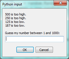
The following program implements a simple guessing game:
This program makes use of the mathematical law of trichotomy (given real numbers a and b, exactly one of these three must be true: a > b, a < b, or a == b).
At line 18 there is a call to the input function, but we don’t do anything with the result, not even assign it to a variable. This is legal in Python. Here it has the effect of popping up the input dialog window and waiting for the user to respond before the program terminates. Programmers often use the trick of doing some extra input at the end of a script, just to keep the window open.
Also notice the use of the message variable, initially an empty string, on lines 6, 12 and 14.
Each time through the loop we extend the message being displayed: this allows us to
display the program’s feedback right at the same place as we’re asking for the next guess.
3.3.14. The continue statement
This is a control flow statement that causes the program to immediately skip the processing of the rest of the body of the loop, for the current iteration. But the loop still carries on running for its remaining iterations:
This prints:
12
16
24
30
done
3.3.15. Paired Data
We’ve already seen lists of names and lists of numbers in Python. We’re going to peek ahead in the textbook a little, and show a more advanced way of representing our data. Making a pair of things in Python is as simple as putting them into parentheses, like this:
We can put many pairs into a list of pairs:
Here is a quick sample of things we can do with structured data like this. First, print all the celebs:
Notice that the celebs list has just 3 elements, each of them pairs.
Now we print the names of those celebrities born before 1980:
This demonstrates something we have not seen yet in the for loop: instead of using a single
loop control variable, we’ve used a pair of variable names, (name, year), instead.
The loop is executed three times — once for each pair in the list, and on each iteration both the
variables are assigned values from the pair of data that is being handled.
3.3.16. Nested Loops for Nested Data
Now we’ll come up with an even more adventurous list of structured data. In this case, we have a list of students. Each student has a name which is paired up with another list of subjects that they are enrolled for:
Here we’ve assigned a list of five elements to the variable students. Let’s print
out each student name, and the number of subjects they are enrolled for:
Python agreeably responds with the following output:
John takes 2 courses
Vusi takes 3 courses
Jess takes 4 courses
Sarah takes 4 courses
Zuki takes 5 courses
Now we’d like to ask how many students are taking CompSci. This needs a counter, and for each student we need a second loop that tests each of the subjects in turn:
The number of students taking CompSci is 3
A more concise of doing this would be the following:
You should set up a list of your own data that interests you — perhaps a list of your CDs, each containing a list of song titles on the CD, or a list of movie titles, each with a list of movie stars who acted in the movie. You could then ask questions like “Which movies starred Angelina Jolie?”
3.3.17. Newton’s method for finding square roots
Loops are often used in programs that compute numerical results by starting with an approximate answer and iteratively improving it.
For example, before we had calculators or computers, people needed to
calculate square roots manually. Newton used a particularly good
method (there is some evidence that this method was known many years before).
Suppose that you want to know the square root of n. If you start
with almost any approximation, you can compute a better approximation (closer
to the actual answer) with the following formula:
Repeat this calculation a few times using your calculator. Can you see why each iteration brings your estimate a little closer? One of the amazing properties of this particular algorithm is how quickly it converges to an accurate answer — a great advantage for doing it manually.
By using a loop and repeating this formula until the better approximation gets close enough to the previous one, we can write a function for computing the square root. (In fact, this is how your calculator finds square roots — it may have a slightly different formula and method, but it is also based on repeatedly improving its guesses.)
This is an example of an indefinite iteration problem: we cannot predict in advance how many times we’ll want to improve our guess — we just want to keep getting closer and closer. Our stopping condition for the loop will be when our old guess and our improved guess are “close enough” to each other.
Ideally, we’d like the old and new guess to be exactly equal to each other when we stop. But exact equality is a tricky notion in computer arithmetic when real numbers are involved. Because real numbers are not represented absolutely accurately (after all, a number like pi or the square root of two has an infinite number of decimal places because it is irrational), we need to formulate the stopping test for the loop by asking “is a close enough to b”? This stopping condition can be coded like this:
Notice that we take the absolute value of the difference between a and b!
This problem is also a good example of when a middle-exit loop is appropriate:
See if you can improve the approximations by changing the stopping condition. Also,
step through the algorithm (perhaps by hand, using your calculator) to see how many
iterations were needed before it achieved this level of accuracy for sqrt(25).
3.3.18. Algorithms
Newton’s method is an example of an algorithm: it is a mechanical process for solving a category of problems (in this case, computing square roots).
Some kinds of knowledge are not algorithmic. For example, learning dates from history or your multiplication tables involves memorization of specific solutions.
But the techniques you learned for addition with carrying, subtraction with borrowing, and long division are all algorithms. Or if you are an avid Sudoku puzzle solver, you might have some specific set of steps that you always follow.
One of the characteristics of algorithms is that they do not require any intelligence to carry out. They are mechanical processes in which each step follows from the last according to a simple set of rules. And they’re designed to solve a general class or category of problems, not just a single problem.
Understanding that hard problems can be solved by step-by-step algorithmic processes (and having technology to execute these algorithms for us) is one of the major breakthroughs that has had enormous benefits. So while the execution of the algorithm may be boring and may require no intelligence, algorithmic or computational thinking — i.e. using algorithms and automation as the basis for approaching problems — is rapidly transforming our society. Some claim that this shift towards algorithmic thinking and processes is going to have even more impact on our society than the invention of the printing press. And the process of designing algorithms is interesting, intellectually challenging, and a central part of what we call programming.
Some of the things that people do naturally, without difficulty or conscious thought, are the hardest to express algorithmically. Understanding natural language is a good example. We all do it, but so far no one has been able to explain how we do it, at least not in the form of a step-by-step mechanical algorithm.
3.4. Some Tips, Tricks, and Common Errors
These are small summaries of ideas, tips, and commonly seen errors that might be helpful to those beginning Python.
3.4.1. Problems with logic and flow of control
We often want to know if some condition holds for any item in a list, e.g. “does the list have any odd numbers?” This is a common mistake:
Can we spot two problems here? As soon as we execute a break, we’ll leave the loop.
So the logic of saying “If I find an odd number I can return True” is fine. However, we cannot
return False after only looking at one item — we can only return False if we’ve been through
all the items, and none of them are odd. So line 10 should not be there, and lines 8 and 9 have to be
outside the loop. Here is a corrected version:
We’ll see This “eureka”, or “short-circuit” style of breaking from a loop as soon as we are certain what the outcome will be again later.
Note that this uses a for ... else construct.
The else clause is executed when a loop has looped without encountering any break statements.
This is ideal for our case here. Also note that the else is not, in this case,
related to the if statement that occurs inside the loop.
It is preferred over this one, which also works correctly:
The performance disadvantage of this one is that it traverses the whole list, even if it knows the outcome very early on.
Tip: Think about the return conditions of the loop
Do I need to look at all elements in all cases? Can I shortcut and take an early exit? Under what conditions? When will I have to examine all the items in the list?
The code in lines 6-9 can also be tightened up. The expression count > 0
itself represents a Boolean value, either True or False (we can say it ‘evaluates’
to either True or False). That True/False value can be used
directly in the print statement. So we could cut out that code and simply
have the following:
Although this code is tighter, it is not as nice as the one that did the short-circuit return as soon as the first odd number was found.
Even shorter:
Tip: Generalize your use of Booleans
Programmers won’t write if is_prime(n) == True: when they could
say instead if is_prime(n): Think more generally about Boolean values,
not just in the context of if or while statements. Like arithmetic
expressions, they have their own set of operators (and, or, not) and
values (True, False) and can be assigned to variables, put into lists, etc.
A good resource for improving your use of Booleans is
http://en.wikibooks.org/wiki/Non-Programmer%27s_Tutorial_for_Python_3/Boolean_Expressions
Exercise time:
- How would we adapt this to print
Trueif all the numbers are odd? Can you still use a short-circuit style? - How would we adapt it to print
Trueif at least three of the numbers are odd? Short-circuit the traversal when the third odd number is found — don’t traverse the whole list unless we have to.
3.4.2. Looping and lists
Computers are useful because they can repeat computation, accurately and fast. So loops are going to be a central feature of almost all programs you encounter.
Tip: Don’t create unnecessary lists
Lists are useful if you need to keep data for later computation. But if you don’t need lists, it is probably better not to generate them.
Here are two functions that both generate ten million random numbers, and return the sum of the numbers. They both work.
What reasons are there for preferring the second version here? (Hint: open a tool like the Performance Monitor on your computer, and watch the memory usage. How big can you make the list before you get a fatal memory error in the first version?)
In a similar way, when working with files, we often have an option to read the whole file contents into a single string, or we can read one line at a time and process each line as we read it. Line-at-a-time is the more traditional and perhaps safer way to do things — you’ll be able to work comfortably no matter how large the file is. (And, of course, this mode of processing the files was essential in the old days when computer memories were much smaller.) But you may find whole-file-at-once is sometimes more convenient!
3.4.3. Glossary
- attribute
- Some state or value that belongs to a particular object. For example,
tesshas a color. - canvas
- A surface within a window where drawing takes place.
- control flow
- See flow of execution.
- for loop
- A statement in Python for convenient repetition of statements in the body of the loop.
- loop body
- Any number of statements nested inside a loop. The nesting is indicated by the fact that the statements are indented under the for loop statement.
- loop variable
- A variable used as part of a for loop. It is assigned a different value on each iteration of the loop.
- instance
- An object of a certain type, or class.
tessandalexare different instances of the classTurtle. - method
- A function that is attached to an object. Invoking or activating the method
causes the object to respond in some way, e.g.
forwardis the method when we saytess.forward(100). - invoke
- An object has methods. We use the verb invoke to mean activate the
method. Invoking a method is done by putting parentheses after the method
name, with some possible arguments. So
tess.forward()is an invocation of theforwardmethod. - module
- A file containing Python definitions and statements intended for use in other
Python programs. The contents of a module are made available to the other
program by using the
importstatement. - object
- A “thing” to which a variable can refer. This could be a screen window, or one of the turtles we have created.
- range
- A built-in function in Python for generating sequences of integers. It is especially useful when we need to write a for loop that executes a fixed number of times.
- terminating condition
- A condition that occurs which causes a loop to stop repeating its body.
In the
forloops we saw in this chapter, the terminating condition has been when there are no more elements to assign to the loop variable. - block
- A group of consecutive statements with the same indentation.
- body
- The block of statements in a compound statement that follows the header.
- Boolean algebra
- Some rules for rearranging and reasoning about Boolean expressions.
- Boolean expression
- An expression that is either true or false.
- Boolean value
- There are exactly two Boolean values:
TrueandFalse. Boolean values result when a Boolean expression is evaluated by the Python interepreter. They have typebool. - branch
- One of the possible paths of the flow of execution determined by conditional execution.
- chained conditional
- A conditional branch with more than two possible flows of execution. In
Python chained conditionals are written with
if ... elif ... elsestatements. - comparison operator
- One of the six operators that compares two values:
==,!=,>,<,>=, and<=. - condition
- The Boolean expression in a conditional statement that determines which branch is executed.
- conditional statement
- A statement that controls the flow of execution depending on some
condition. In Python the keywords
if,elif, andelseare used for conditional statements. - logical operator
- One of the operators that combines Boolean expressions:
and,or, andnot. - nesting
- One program structure within another, such as a conditional statement inside a branch of another conditional statement.
- prompt
- A visual cue that tells the user that the system is ready to accept input data.
- truth table
- A concise table of Boolean values that can describe the semantics of an operator.
- type conversion
- An explicit function call that takes a value of one type and computes a corresponding value of another type.
- algorithm
- A step-by-step process for solving a category of problems.
- body
- The statements inside a loop.
- bump
- Programmer slang. Synonym for increment.
- continue statement
- A statement that causes the remainder of the current iteration of a loop to be skipped. The flow of execution goes back to the top of the loop, evaluates the condition, and if this is true the next iteration of the loop will begin.
- counter
- A variable used to count something, usually initialized to zero and incremented in the body of a loop.
- cursor
- An invisible marker that keeps track of where the next character will be printed.
- decrement
- Decrease by 1.
- definite iteration
- A loop where we have an upper bound on the number of times the
body will be executed. Definite iteration is usually best coded
as a
forloop. - escape sequence
- An escape character, \, followed by one or more printable characters used to designate a nonprintable character.
- increment
- Both as a noun and as a verb, increment means to increase by 1.
- infinite loop
- A loop in which the terminating condition is never satisfied.
- indefinite iteration
- A loop where we just need to keep going until some condition is met.
A
whilestatement is used for this case. - initialization (of a variable)
- To initialize a variable is to give it an initial value. Since in Python variables don’t exist until they are assigned values, they are initialized when they are created. In other programming languages this is not the case, and variables can be created without being initialized, in which case they have either default or garbage values.
- iteration
- Repeated execution of a set of programming statements.
- loop
- The construct that allows allows us to repeatedly execute a statement or a group of statements until a terminating condition is satisfied.
- loop variable
- A variable used as part of the terminating condition of a loop.
- meta-notation
- Extra symbols or notation that helps describe other notation. Here we introduced square brackets, ellipses, italics, and bold as meta-notation to help describe optional, repeatable, substitutable and fixed parts of the Python syntax.
- middle-test loop
- A loop that executes some of the body, then tests for the exit condition,
and then may execute some more of the body. We don’t have a special
Python construct for this case, but can
use
whileandbreaktogether. - nested loop
- A loop inside the body of another loop.
- newline
- A special character that causes the cursor to move to the beginning of the next line.
- post-test loop
- A loop that executes the body, then tests for the exit condition. We don’t have a special
Python construct for this, but can use
whileandbreaktogether. - pre-test loop
- A loop that tests before deciding whether the execute its body.
forandwhileare both pre-test loops. - tab
- A special character that causes the cursor to move to the next tab stop on the current line.
- trichotomy
- Given any real numbers a and b, exactly one of the following relations holds: a < b, a > b, or a == b. Thus when you can establish that two of the relations are false, you can assume the remaining one is true.
- trace
- To follow the flow of execution of a program by hand, recording the change of state of the variables and any output produced.
3.4.4. Exercises
Assume the days of the week are numbered 0,1,2,3,4,5,6 from Sunday to Saturday. Write a program that asks a day number, and prints the day name (a string).
You go on a wonderful holiday (perhaps to jail, if you don’t like happy exercises) leaving on day number 3 (a Wednesday). You return home after 137 sleeps. Write a general version of the program which asks for the starting day number, and the length of your stay, and it will tell you the name of day of the week you will return on.
Give the logical opposites of these conditions
a > ba >= ba >= 18 and day == 3a >= 18 and day != 3
What do these expressions evaluate to?
3 == 33 != 33 >= 4not (3 < 4)
Complete this truth table:
p q r (not (p and q)) or r F F F ? F F T ? F T F ? F T T ? T F F ? T F T ? T T F ? T T T ? Write a program which is given an exam mark, and it returns a string — the grade for that mark — according to this scheme:
Mark Grade >= 75 First [70-75) Upper Second [60-70) Second [50-60) Third [45-50) F1 Supp [40-45) F2 < 40 F3 The square and round brackets denote closed and open intervals. A closed interval includes the number, and open interval excludes it. So 39.99999 gets grade F3, but 40 gets grade F2. Assume
numbers = [83, 75, 74.9, 70, 69.9, 65, 60, 59.9, 55, 50,
                     49.9, 45, 44.9, 40, 39.9, 2, 0]
Test your code by printing the mark and the grade for all the elements in this list.
Write a program which, given the length of two sides of a right-angled triangle, returns the length of the hypotenuse. (Hint:
x ** 0.5will return the square root.)Write a program which, given the length of three sides of a triangle, will determine whether the triangle is right-angled. Assume that the third argument to the function is always the longest side. It will return
Trueif the triangle is right-angled, orFalseotherwise.Hint: Floating point arithmetic is not always exactly accurate, so it is not safe to test floating point numbers for equality. If a good programmer wants to know whether
xis equal or close enough toy, they would probably code it up as:threshold = 1e-7 if abs(x-y) < threshold: # If x is approximately equal to y ...
Extend the above program so that the sides can be given to the function in any order.
If you’re intrigued by why floating point arithmetic is sometimes inaccurate, on a piece of paper, divide 10 by 3 and write down the decimal result. You’ll find it does not terminate, so you’ll need an infinitely long sheet of paper. The representation of numbers in computer memory or on your calculator has similar problems: memory is finite, and some digits may have to be discarded. So small inaccuracies creep in. Try this script:
Write a program that prints
We like Python's turtles!1000 times.- Write a program that uses a for loop to print
One of the months of the year is JanuaryOne of the months of the year is February…
Suppose our turtle
tessis at heading 0 — facing east. We execute the statementtess.left(3645). What doestessdo, and what is her final heading?Assume you have the assignment
numbers = [12, 10, 32, 3, 66, 17, 42, 99, 20]- Write a loop that prints each of the numbers on a new line.
- Write a loop that prints each number and its square on a new line.
- Write a loop that adds all the numbers from the list into a variable called total.
You should set the total variable to have the value 0 before you start adding them up,
and print the value in
totalafter the loop has completed. - Print the product of all the numbers in the list. (product means all multiplied together)
Use
forloops to make a turtle draw these regular polygons (regular means all sides the same lengths, all angles the same):- An equilateral triangle
- A square
- A hexagon (six sides)
- An octagon (eight sides)
A drunk pirate makes a random turn and then takes 100 steps forward, makes another random turn, takes another 100 steps, turns another random amount, etc. A social science student records the angle of each turn before the next 100 steps are taken. Her experimental data is
[160, -43, 270, -97, -43, 200, -940, 17, -86]. (Positive angles are counter-clockwise.) Use a turtle to draw the path taken by our drunk friend.Enhance your program above to also tell us what the drunk pirate’s heading is after he has finished stumbling around. (Assume he begins at heading 0).
If you were going to draw a regular polygon with 18 sides, what angle would you need to turn the turtle at each corner?
At the interactive prompt, anticipate what each of the following lines will do, and then record what happens. Score yourself, giving yourself one point for each one you anticipate correctly:
>>> import turtle
>>> window = turtle.Screen()
>>> tess = turtle.Turtle()
>>> tess.right(90)
>>> tess.left(3600)
>>> tess.right(-90)
>>> tess.speed(10)
>>> tess.left(3600)
>>> tess.speed(0)
>>> tess.left(3645)
>>> tess.forward(-100)
Write a program to draw a shape like this:

Hints:
- Try this on a piece of paper, moving and turning your cellphone as if it was a turtle. Watch how many complete rotations your cellphone makes before you complete the star. Since each full rotation is 360 degrees, you can figure out the total number of degrees that your phone was rotated through. If you divide that by 5, because there are five points to the star, you’ll know how many degrees to turn the turtle at each point.
- You can hide a turtle behind its invisibility cloak if you don’t want it shown. It will still
draw its lines if its pen is down. The method is invoked as
tess.hideturtle(). To make the turtle visible again, usetess.showturtle().
Write a program to draw a face of a clock that looks something like this:
Create a turtle, and assign it to a variable. When you ask for its type, what do you get?
This chapter showed us how to sum a list of items,
and how to count items. The counting example also had an if statement
that let us only count some selected items. we have break to exit a loop, and
continue to abandon the current iteration of the loop without ending the loop.
Composition of list traversal, summing, counting, testing conditions and early exit is a rich collection of building blocks that can be combined in powerful ways to create many functions that are all slightly different.
The first six questions are typical functions you should be able to write using only these building blocks.
Write a program to count how many odd numbers are in a list.
Sum up all the even numbers in a list.
Sum up all the negative numbers in a list.
Count how many words in a list have length 5.
Sum all the elements in a list up to but not including the first even number. (What if there is no even number?)
Count how many words occur in a list up to and including the first occurrence of the word “sam”. (What if “sam” does not occur?)
Add a print function to Newton’s
sqrtalgorithm that prints outbettereach time it is calculated. Call your modified program with 25 as an argument and record the results.Write a program that prints out the first n triangular numbers. A call to with
n = 5would produce the following output:1 1 2 3 3 6 4 10 5 15
(hint: use a web search to find out what a triangular number is.)
Write a program which prints
Truewhennis a prime number andFalseotherwise.Revisit the drunk pirate problem. This time, the drunk pirate makes a turn, and then takes some steps forward, and repeats this. Our social science student now records pairs of data: the angle of each turn, and the number of steps taken after the turn. Her experimental data is [(160, 20), (-43, 10), (270, 8), (-43, 12)]. Use a turtle to draw the path taken by our drunk friend.
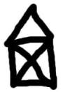
Many interesting shapes can be drawn by the turtle by giving a list of pairs like we did above, where the first item of the pair is the angle to turn, and the second item is the distance to move forward. Set up a list of pairs so that the turtle draws a house with a cross through the centre, as show here. This should be done without going over any of the lines / edges more than once, and without lifting your pen.
Recall the digit counting program. What will it print with
n = 0? Modify it to print1for this case. Why does a call withn = -24result in an infinite loop? (hint: -1//10 evaluates to -1) Modifynum_digitsso that it works correctly with any integer value.Write a program that counts the number of even digits in
n.Write a program that computes the sum of the squares of the numbers in the list
numbers. For example a call with,numbers = [2, 3, 4]should print 4+9+16 which is 29.