Fitting¶

Suppose we want to determine the gravitational acceleration. To this end, we could drop an object from the building and measure how long it takes for the object to reach the ground with a stopwatch. Newton’s laws predict the following model:

$h = \frac{1}{2} g t^2$

where $h$ is the height from which we dropped the object, and $t$ the time it takes to hit the ground. So from our one measurement we could now calculate the gravitational acceleration $g$ .

We can measure the height very accurately, but since we use a stopwatch to measure time, that value is a lot less reliable because you might have started and stopped your stopwatch at the wrong moments. Therefore, the result will not be very accurate. To make the value more accurate we should repeat the same measurement $n$ times to obtain an average $t$ and use that instead. We’ll get back to this later.

For now we are more interested in the question: is this model correct? To test this question, we drop our object from different heights, doing multiple measurements for each height to get reliable values. The data, obtained by simulation for health and safety reasons, are given in the following table:

y	t	n
10	1.4	5
20	2.1	3
30	2.6	8
40	3.0	15
50	3.3	30

Since the model predicts a parabola, we want to fit the data to this model to see how good it works. It might be a bit confusing, but $h$ is our x axis, and $t$ is the y axis.

We use the symfit package to do our fitting. You can find the installation instructions here.

To fit the data to the model we run the following code:

import numpy as np
from symfit import Variable, Parameter, Fit, Model, sqrt

t_data = np.array([1.4, 2.1, 2.6, 3.0, 3.3])
h_data = np.array([10, 20, 30, 40, 50])

# We now define our model
h = Variable('h')
t = Variable('t')
g = Parameter('g')

t_model = Model({t: sqrt(2 * h / g)})

fit = Fit(t_model, h=h_data, t=t_data)
fit_result = fit.execute()
print(fit_result)

Looking at these results, we see that 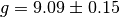$g = 9.09 \pm 0.15$ for this dataset. In order to plot this result alongside the data, we need to calculate values for the model. In the same script, we can do:

# Make an array from 0 to 50 in 1000 steps
h_range = np.linspace(0, 50, 1000)
fit_data = t_model(h=h_range, g=fit_result.value(g))
t_fit = fit_data.t
Note

When calling a symfit.Model, a namedtuple is returned with all the components of the model evaluated. In this case there is only one component, and can be accessed by requesting fit_data.t or fit_data[0].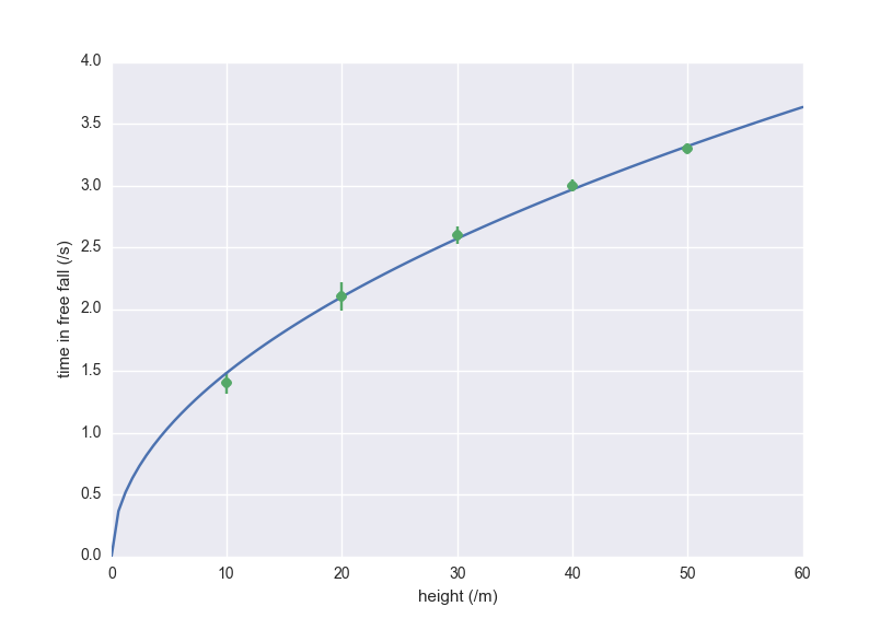

This gives the model evaluated at all the points in h_range. Making the actual plot is left to you as an exercise. We see that we can request the fitted value of g by calling fit_result.value(g), which returns $9.09$ .

Let’s think for a second about the implications. The value of $g$ is $g = 9.81$ in the Netherlands. Based on our result, the textbooks should be rewritten because that value is extremely unlikely to be true given the small standard deviation in our data. It is at this point that we remember that our data point were not infinitely precise: we took many measurements and averaged them. This means there is an uncertainty in each of our data points. We will now account for this additional uncertainty and see what this does to our conclusion. To do this we first have to describe how the fitting actually works.

How does it work?¶

In fitting we want to find values for the parameters such that the differences between the model and the data are as small as possible. The differences (residuals) are easy to calculate:

$f(x_i, \vec{p}) - y_i$

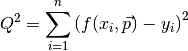
Here we have written the parameters as a vector $\vec{p}$ , to indicate that we can have multiple parameters. $x_i$ and $y_i$ are the x and y coordinates of the i’th datapoint. However, if we were to minimize the sum over all these differences we would have a problem, because these differences can be either possitive or negative. This means there’s many ways to add these values and get zero out of the sum. We therefore take the sum over the residuals squared:

$Q^2 = \sum_{i=1}^n \left(f(x_i, \vec{p}) - y_i\right)^2$

Now if we minimize $Q^2$ , we get the best possible values for our parameters. The fitting algorithm actually just takes some values for the parameters, calculates $Q^2$ , then changes the values slightly by adding or subtracting a number, and checks if this new value is smaller than the old one. If this is true it keeps going in the same direction until the value of $Q^2$ starts to increase. That’s when you know you’ve hit a minimum. Of cource the trick is to do this smartly, and a lot of algorithms have been developed in order to do this.

Propagating Uncertainties¶

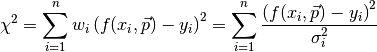
In the example above we the fitting process assumed that every measurement was equally reliable. But this is not true. By repeating a measurement and averaging the result, we can improve the accuracy. So in our example, we dropped our object from every height a couple of times and took the average. Therefore, we want to assign a weight depending on how accurate the average value for that height is. Statistically the weight $w_i$ to use is $w_i = \frac{1}{\sigma_i^2}$ , where $\sigma_i$ is the standard deviation for each point.

Our sum to minimize now changes to:

$\chi^2 = \sum_{i=1}^n w_i \left(f(x_i, \vec{p}) - y_i\right)^2 = \sum_{i=1}^n \frac{ \left(f(x_i, \vec{p}) - y_i\right)^2}{\sigma_i^2}$

But how do we know the standard deviation in the mean value we calculate for every height? Suppose the standard deviation of our stopwatch is $\sigma_{stopwatch}=0.2$ . If we do $n$ measurements from the same height, the average time is found by calculating

$\bar{t} = \frac{1}{n} \sum_{i=1}^n t_i$

It can be shown that the standard deviation of the mean is now:

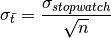
$\sigma_{\bar{t}} = \frac{\sigma_{stopwatch}}{\sqrt{n}}$

So we see that by increasing the amount of measurements, we can decrease the uncertainty in $\bar{t}$ . Our simulated data now changes to:

y	t	n	$\sigma_t$
10	1.4	5	0.089
20	2.1	3	0.115
30	2.6	8	0.071
40	3.0	15	0.052
50	3.3	30	0.037

The values of $\sigma_t$ have been calculated by using the above formula. Let’s fit to this new data set using symfit. Notice that there are some small differences to the code:

import numpy as np
from symfit import Variable, Parameter, Fit, Model, sqrt

t_data = np.array([1.4, 2.1, 2.6, 3.0, 3.3])
h_data = np.array([10, 20, 30, 40, 50])
n = np.array([5, 3, 8, 15, 30])
sigma = 0.2
sigma_t = sigma / np.sqrt(n)

# We now define our model
h = Variable('h')
t = Variable('t')
g = Parameter('g')
t_model = Model({t: sqrt(2 * h / g)})

fit = Fit(t_model, h=h_data, t=t_data, sigma_t=sigma_t)
fit_result = fit.execute()
print(fit_result)

Note

Looking at the initiation of Fit, we see that uncertainties can be provided to Variable’s by prepending their name with sigma_, in this case sigma_t.

Including these uncertainties in the fit yields $g = 9.10 \pm 0.16$ . The accepted value of $g = 9.81$ is well outside the uncertainty in this data. Therefore the textbooks must be rewriten!

This example shows the importance of propagating your errors consistently. (And of the importance of performing the actual measurement as the author of a chapter on error propagation so you don’t end up claiming the textbooks have to rewritten.)

More on symfit¶

There are a lot more features in symfit to help you on your quest to fitting the universe. You can find the tutorial here.

It is recommended you read this as well before starting to fit your own data.